Multivariate Gaussian distributions have many computationally favorable properties that have been used extensively in robotics.
In this exercise, we focus on some operations with Gaussian densities that result in another Gaussian density, namely,
linear combination and product of Gaussians. We will see how one can use these operations in regression problems.
1. Multivariate Gaussian Distribution
Fill in the code below to implement linear_combination and product_gaussians.
def gaussian_nD(x, mu, sigma):
D = x.shape[0]
cons = ((2*np.pi)**(-D/2)) * (np.linalg.det(sigma)**(-0.5))
return cons*np.exp(-0.5*(x-mu).dot(np.linalg.inv(sigma))@ (x-mu))
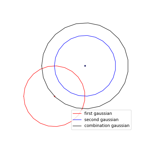
def linear_combination(A1, A2, c, mu1, mu2, sigma1, sigma2):
mu_L = np.zeros(2) # Implement here
sigma_L = np.eye(2) # Implement here
return mu_L, sigma_L
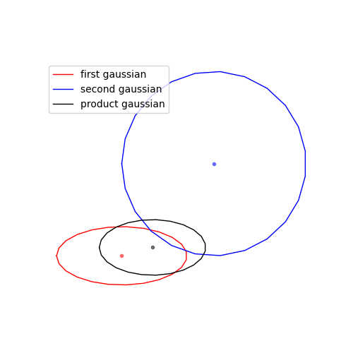
def product_gaussians(mu1, mu2, sigma1, sigma2):
sigma1_inv = np.linalg.inv(sigma1)
sigma2_inv = np.linalg.inv(sigma2)
sigma_P = np.eye(2)# Implement here
mu_P = np.zeros(2) # Implement here
c = 0. # Implement here
return mu_P, sigma_P, c
You have access to a plotting function called plot_gaussian(mu, sigma, ax, dim=None, color='r', alpha=0.5, lw=1, markersize=6, **kwargs).
You need to give mu : ndarray(N,) , sigma : ndarray(N,N) and ax : subplot object
to the function (you can also give other arguments that matplotlib accepts).
Implement product_gaussians in the code above and run the code below to test your answer. You can verify your answer by clicking on the button below the code.
Implement linear_combination in the code above and run the code below to test your answer. You can verify your answer by clicking on the button below the code (the plot in the answer is generated with c=0).
2. Fitting a Gaussian distribution to demonstrations
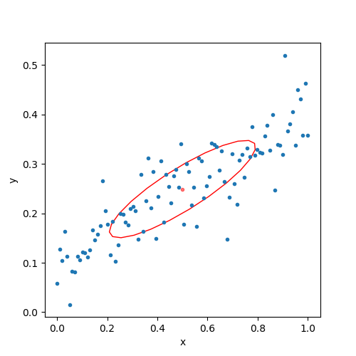
Given a dataset X with \bm{X} \in \mathcal{R}^{2\times\mathrm{nb\_data}}, implement a function fit_gaussian that fits a Gaussian distribution onto this dataset and returns its mean and covariance.
def fit_gaussian(X):
mu = np.zeros(2) # implement here
sigma = np.eye(2) # implement here
return mu, sigma
Verify your function by plotting the resulting Gaussian distribution along with the dataset. To do this, you can run the code below by changing the noise level.
You can also click on the button below to verify your answer (the answer is generated with noise_scale=0.01).
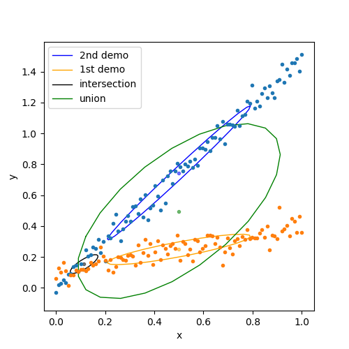
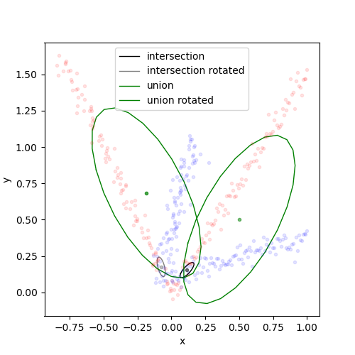
We are given two different sets of demonstration data, each represented by a Gaussian distribution. Depending on the application, we may be interested
only in capturing the common parts in both demonstrations, which we will call intersection, or capturing both demonstration datasets together,
which we will call union. Intersection and union correspond to the functions that we implemented in this session.
Which ones do you think fit to these specifications?
# Create a new dataset X2
x2 = np.linspace(0,1,nb_data)
y2 = 1.5*x2 + np.random.randn(nb_data)*noise_scale
X2 = np.stack([x2,y2])
# Fit another Gaussian distribution
mu2, sigma2 = fit_gaussian(X2)
# Compute the resulting Gaussian for the intersection case
mu_intersection, sigma_intersection = np.zeros(2), np.eye(2) # implement here
# Compute the resulting Gaussian for the union case
mu_union, sigma_union = np.zeros(2), np.eye(2) # implement here
# Create a new dataset X2
x2 = np.linspace(0,1,nb_data)
y2 = 1.5*x2 + np.random.randn(nb_data)*noise_scale
X2 = np.stack([x2,y2])
# Fit another Gaussian distribution
mu2, sigma2 = fit_gaussian(X2)
# Compute the resulting Gaussian for the intersection case
mu_intersection, sigma_intersection, c = product_gaussians(mu1, mu2, sigma1, sigma2) # implement here
# Compute the resulting Gaussian for the union case
mu_union, sigma_union = fit_gaussian(np.concatenate([X1, X2], axis=-1)) # implement here
Plot these Gaussian distributions to verify your results with the button below.
Now consider the case where our coordinate system is rotated \pi/3 radians counterclockwise, which also rotated our dataset. Instead of refitting a distribution onto this new rotated dataset, we would like to reuse the mu_union, sigma_union and mu_intersection, sigma_intersection and the rotation matrix R to encode our new rotated dataset.
One function implemented in this section can accomplish this. Call this function with the appropriate arguments and plot the results. You can verify your answer with the button below the code (that you can also use as a hint).